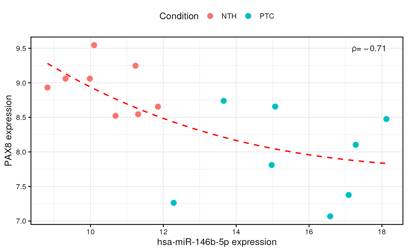
Plot correlation between miRNAs and genes within biological groups

This function creates a scatter plot that shows the correlation between miRNA and gene expression levels. This is useful after correlation analysis performed through the mirnaIntegration() function, to graphically visualize the quantitative effect of miRNA dysregulations on target gene expression. Furthermore, this function performs linear/monotonic regression to better represent the relationships between miRNA-target pairs.

Usage

plotCorrelation(
  mirnaObj,
  mirna,
  gene,
  condition = NULL,
  showCoeff = TRUE,
  regression = TRUE,
  useRanks = FALSE,
  lineCol = "red",
  lineType = "dashed",
  lineWidth = 0.8,
  pointSize = 3,
  colorScale = NULL,
  fontSize = 12,
  fontFamily = "",
  legend = "top",
  borderWidth = 1,
  allBorders = TRUE,
  grid = TRUE
)

Arguments

mirnaObj: A MirnaExperiment object containing miRNA and gene data
mirna: The name of the miRNA for which we want to observe the correlation
gene: The name of the gene for which we want to observe the correlation
condition: It must be NULL (default) to plot expression based on the group variable used for differential expression analysis. Alternatively, it must be a character/factor object that specifies group memberships (eg. c("healthy, "healthy", "disease", "disease"))
showCoeff: Logical, whether to show the correlation coeffficient or not. Note that the "R" is used for Pearson's correlation", "rho" for Spearman's correlation, and "tau" for Kendall's correlation. Default is TRUE
regression: Logical, whether to display a linear/monotonic regression line that fits miRNA-gene correlation data. Default is TRUE
useRanks: Logical, whether to represent non-parametric correlation analyses (Spearman's and Kendall's correlations) through rank-transformed data. Note that in this case, linear regression is performed on ranked data instead of monotonic regression. Default is FALSE
lineCol: It must be an R color name that specifies the color of the regression line. Default is red. Available color formats include color names, such as 'blue' and 'red', and hexadecimal colors specified as #RRGGBB
lineType: It specifies the line type used for the regression line. It must be either 'blank', 'solid', 'dashed' (default), 'dotted', 'dotdash', 'longdash' or 'twodash'
lineWidth: The width of the fitted regression line (default is 0.8)
pointSize: The size of points in the correlation plot (default is 3)
colorScale: It must be a named character vector where values correspond to R colors, while names coincide with the groups specified in the condition parameter (eg. c("healthy" = "green", "disease" = "red")). Default is NULL, in order to use the default color scale. Available color formats include color names, such as 'blue' and 'red', and hexadecimal colors specified as #RRGGBB
fontSize: The base size for text elements within the plot. Default is 12
fontFamily: The base family for text elements within the plot
legend: The position of the legend. Allowed values are top, bottom, right, left and none. The default setting is top to show a legend above the plot. If none is specified, the legend will not be included in the graph.
borderWidth: The width of plot borders (default is 1)
allBorders: Logical, whetether to show all panel borders, or just the bottom and left borders. Default is TRUE
grid: Logical, whether to show grid lines or not. Default is TRUE

Value

An object of class ggplot containing the correlation scatter plot.

Details

When non-parametric correlation has been performed with the mirnaIntegration() function, a regression line can be fitted through monotonic regression on expression levels, or through linear regression performed on rank-transformed data. Since, ranks do not correspond to real expression values, the default option is to perform monotonic regression to fit a monotonic curve. To do so, this function makes use of the MonoPoly R package, which implements the algorithm proposed by Murray et al. in 2016.

References

K. Murray, S. Müller & B. A. Turlach (2016) Fast and flexible methods for monotone polynomial fitting, Journal of Statistical Computation and Simulation, 86:15, 2946-2966, DOI: 10.1080/00949655.2016.1139582.

Author

Jacopo Ronchi, jacopo.ronchi@unimib.it

Examples

# load example MirnaExperiment object
obj <- loadExamples()

# plot correlation between miR-146b and PAX8 with monotonic regression curve
plotCorrelation(obj, "hsa-miR-146b-5p", "PAX8", condition = "disease")